[판다스] matplotlib을 이용한 그래프 그리기: 히스토그램, 산점도 그래프 - <Do it! 데이터 분석을 위한 판다스 입문> 실습
[ matplotlib 을 이용해서 그래프 그리기 ]
데이터셋 불러오기
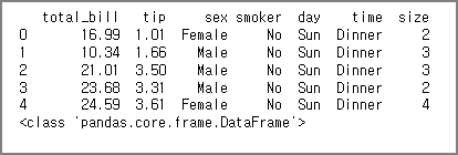
먼저 seaborn 라이브러리에 내장되어 있는 tips 데이터셋을 불러온다.
그리고 tips에 어떤 데이터가 들어있는지 확인해보았다.
import seaborn as sns

tips = sns.load_dataset('tips')

print(tips.head())
print(type(tips))
아래와 같은 데이터가 들어있고, dtype은 data frame 이다.
7개의 column이 있음을 확인할 수 있다.
히스토그램 - 단변량 그래프
가장 단순한 형태의 변수가 하나인 단변량 그래프를 그려보자.
단변량 히스토그램은 간단하기 때문에 추가적인 설명은 생략한다.
import matplotlib.pyplot as plt
%matplotlib inline

fig = plt.figure()
axes = plt.subplot(1,1,1)📌%matplotlib inline :
Literally used to display Matplotlib charts inline. Static images of your plots are embedded in the notebook.
(*TMI : inline = '그때마다 즉시 처리하는' 이라는 뜻이 있다.)
*비교! ➡️ %matplotlib notebook :
Interactive plots are embedded within the notebook, which allows you to zoom, pan, and save your plots.
axes1.hist(tips['total_bill'])
axes1.set_title('Histogram of Total Bill')
axes1.set_xlabel('Total Bill')
axes.set_ylabel('Frequency')

print(fig)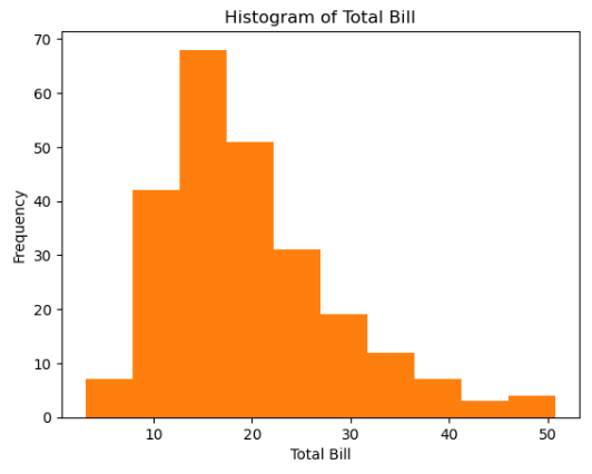
산점도 그래프 - 이변량 그래프
이번에는 matplotlib의 scatter() 함수를 이용해서 산점도 그래프를 그려보자.
*TMI : scatter = 영어로 '흩뿌리다' 라는 뜻이다. 물감을 후두둑 흩뿌리듯이.. 딱 산점도 그래프처럼!
(이렇게 직관적으로 지어진 함수명을 만나면 영어쟁이는 기분이 좋다ㅎㅎ)
scatter_graph = plt.figure()
axes1 = scatter_graph.add_subplot(1,1,1)

axes1.scatter(tips['total_bill'], tips['tip']
axes1.set_title('Scatter Plot of Total Bill & Tip)
axes1.set_xlabel('Total Bill')
axes1.set_ylabel('Tip')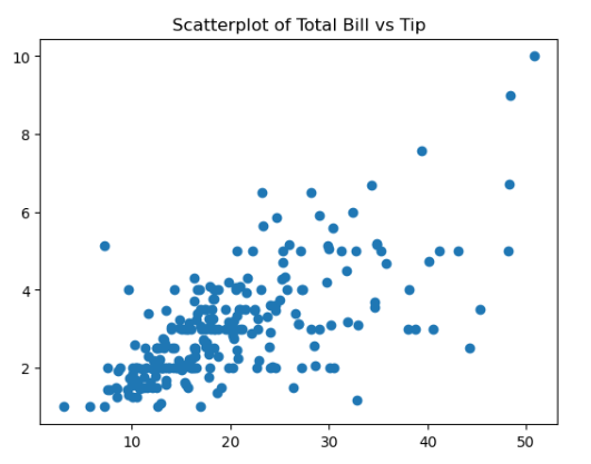
박스 그래프 - 이변량 그래프
boxplot() 함수를 이용하면 박스 플롯을 만들 수 있다.
box = plt.figure()
axes1 = box.add_subplot(1,1,1)

axes1.boxplot(
    [tips[tips['sex'] == 'Female']['tip'],
     tips[tips['sex'] == 'Male']['tip']],
    labels = ['Female','Male']
)

axes1.set_title('Boxplot of Tips by Sex')
axes1.set_xlabel('Sex')
axes1.set_ylabel('Tip')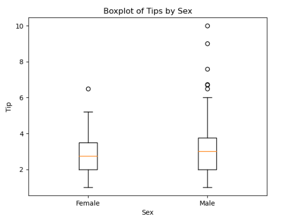
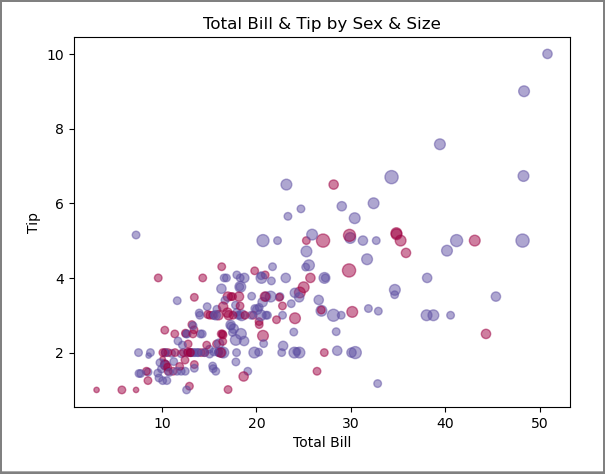
산점도 그래프 - 다변량 그래프 (★ ★ ★)
다변량 그래프에서는 3개 이상의 변수를 사용해서 그래프를 그린다.
점의 크기를 다르게 하거나, 점의 투명도를 조절해서 여러 변수들을 구별하여 사용할 수 있다.
tips 데이터셋의 tip과 total bill로 산점도를 그려볼텐데,
이 때 성별에 따라 색깔을 다르게 표현해보겠다.
다만 Female, Male은 문자열이므로 색상을 지정하는 값이 될 수 없기에
0,1의 정수형으로 치환하는 함수를 생성한다.
def sex_code(sex) :
	if sex == 'Female' :
    	return 0
    else :
    	return 1
sex_code 가 반환한 정수형 값들은 data frame에 sex_code라는 컬럼을 새로 만들어서 추가한다.
head() 를 이용해서 확인해보면, 컬럼이 잘 생성되어 데이터들이 저장된 것이 보인다.
(*참고 : apply 메서드는 'sex_code' 함수를 'sex' 컬럼에 브로드캐스팅하기 위해 사용했다.)
tips['sex_code'] = tips['sex'].apply(sex_code)

tips.head(2)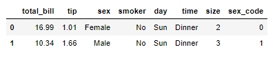
이제 위에서 다뤘던 scatter() 을 이용해 그래프를 그려보자.
📌 scatter() parameters :
- c : 점의 색상 (marker color)
- s : 점의 크기 (marker size)
- alpha : 점의 투명도 (blending value, between 0: transparent ~ 1:opaque)
- cmap : 컬러맵 (colormap instance or registered colormap name used to map scalar data to colors)
scattered = plt.figure()
axes1 = scattered.add_subplot(1,1,1)

axes1.scatter(
        x = tips['total_bill'],
        y = tips['tip'],
        c = tips['sex_code'],
        s = tips['size'] * 15,
        alpha = 0.5,
        cmap = 'Spectral'
)

axes1.set_title('Total Bill & Tip by Sex & Size')
axes1.set_xlabel('Total Bill')
axes1.set_ylabel('Tip')